System evolution and reliability of systems
0. Foreword
The content of this page has first been published in :
- Crevecoeur, G.U., "A Model for the Integrity Assessment of Ageing
Repairable Systems", IEEE Trans. Reliability, 42(1), 1993, pp. 148-155
- Crevecoeur, G. U., "Reliability assessment of ageing operating
systems", Eur. J. Mech. Eng., 39(4), 1994, pp. 219-228 - A copy of this article can be found
here.
1. Learning curve
Starting with Duane's investigations (Duane,1964), we observe that for several repairable systems - hydromechanical devices, airplane generators, submarine diesel engines, loading cranes (Bassin,1969)and army trucks (Bell & Miodusky,1976)-, the failure rate may be described by equation (3). An example of the corresponding curve is shown in Figure 19. Duane called this the "learning curve".
The learning curve can be compared to the hazard rate curve for a Weibull distribution with parameter "b"
less than 1. Indeed, the 2-parameter Weibull distribution is given by equation (5). The corresponding hazard rate (or "conditional failure rate") is given by equation
(6) which is equivalent to equation (3).
The integral of equation (3) gives, by definition, the cumulative number of failures, which can be considered the simplest parameter reflecting the ageing or evolution of the system. If the probability of system failure is attached to the internal non-standard responses, one would say that the learning curve reflects the hazard rate due to the failure-inducing non-standard responses, which would correspond to a Weibull distribution with "b" less than 1. This is in full agreement with the existence of negative feedback loops since a decreasing hazard rate means that the system adapts to its operating conditions. The observed learning curve is thus an experimental confirmation of the existence of negative feedback loops in the ageing or evolution of systems.
2. Bathtub curve
However, many cases of systems have also been observed for which the failure rate was constant or increased. For this last case, following equation was proposed by Cox & Lewis (1966) :

It was successfully applied to aircraft air conditioners (Lawless,1982), submarine main propulsion diesel engines failures (Ascher &
Feingold,1969), etc.
When combined with the learning curve, the behaviour described by equation (RL 01) plots as what is often called a "bathtub curve". This curve shows three successive stages: (1) one learning stage as described by Duane, followed by (2) a period with constant failure rate interpreted as corresponding to random failures, and (3) a final stage with an increase in the failure rate due to wear out phenomena.
Lee (1980) proposed the following equation to describe the bathtub curve:

which reduces to equation (RL 01) when b=1 and to equation (3) when a=0. If a1 and b are positive and b is less than 1, one gets a bathtub curve.
Because "l1,2" is a rate, equation (RL 02) is to be appropriately integrated with respect to time. Moreover, the integral of the bathtub curve must be a curve showing a first concave (from below) part followed by a convex (from below) part, both parts being separated by an intermediate, quasi-straight linear zone of variable length. It is difficult, if not impossible, to find a function describing such a curve while having a derivative given by equation (RL 02).
However, if we observe that "l1,2" can be considered the first term [v.(du/dt)] of a full derivative [d(u.v)/dt], of which the second term [u.(dv/dt)] is given by:

then 3 interesting results are obtained:
 The full derivative l4=l1,2+l3 can also be used to fit the bathtub curve ;
Express l4 as:
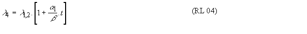
l4reduces to equation (3) when a1=0, and to equation (RL 01) when b=1 and "a1.t" is small, as (1+a1.t) is about exp(a1.t).
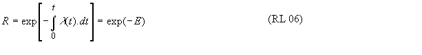
Integrating "l4" now becomes very easy, and, with the reasonable assumption that E(0)=0, we obtain:

which is Equation
E-1.
By comparison to the Weibull distribution, we can define a modified Weibull distribution from E(t)as given by Equation E-1 and l(t)=dE/dt. Following classical reliability parameters can then be computed: R(t), F(t) and f(t). As before, a "." above the parameter means "time derivative".
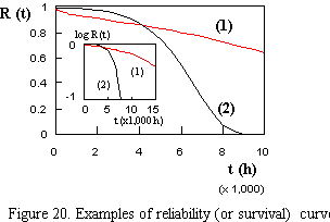
The "reliability R(t)" will be given by definition by:
and corresponds to following figure:
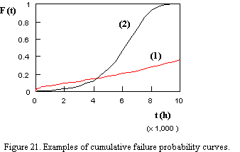
The "cumulative probability of failure F(t)" is given by:

and corresponds to following figure:
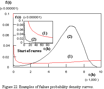
The "failure probability density f(t)" is given by:

and corresponds to following figure:
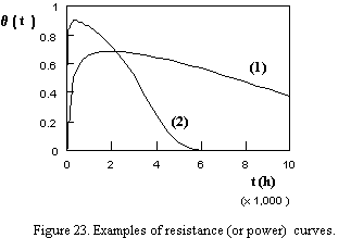
Finally, it is noteworthy that the inverse of the exponential of the bathtub curve also gives an experimentally observed curve which could be called the "resistance curve q". See equation and corresponding figure hereafter:

The only differences between the modified Weibull distribution used for the present class of
systems and the Weibull distribution are: (1) the presence of an additional factor exp(a.t) and (2) the restriction that "b" is less than 1. To return to a Weibull distribution, it is sufficient to make a=0 in above equations.
Back to Home page

Page last revised: March 26th,
2016
Best viewed with Explorer
© All rights reserved
- Sysev (Belgium) 15/03/98